Accessibility
Accessible Excel Spreadsheets
Last modified 2/16/2022
Use the following steps to create a spreadsheet in Microsoft Excel so it is accessible to all users.
Delete Unused Worksheets
Any unused worksheets should be deleted from the workbook.
Step 1. Right Click on Worksheet Tab
Step 2. Choose Delete

Add a Title to Workbook
All documents should have a meaningful title add which represents its content.
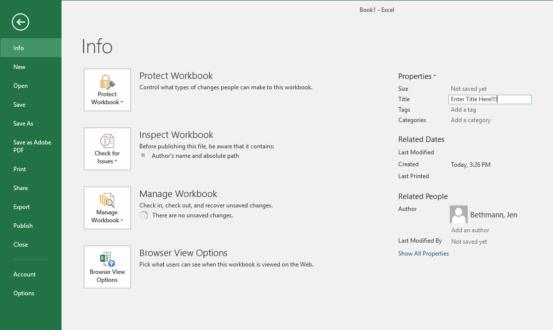
Step 1. Select File then Info.
Open your Excel spreadsheet and select File from the Main Tabs then select Info from the list of items on the left side of the screen.
Step 2. Type Title.
On the Info screen, type your descriptive title into the text field marked Title.
Adding Titles to Worksheets
Each worksheet needs to have a distinctive title which references the spreadsheet's content. "Sheet 1" and "Sheet 2" are not considered descriptive titles.
Step 1. Select the worksheet tab.
To add a title to the worksheet, double click on the worksheet tab or use the keystrokes Alt+O, H, R.
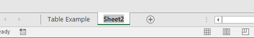
Step 2. Type worksheet title.
Type in descriptive title then press enter to move focus off the renamed tab. Title all worksheet titles in a workbook should be unique values.
Colors Styles
Be careful choosing color styles on your table. Make sure you do not present color as the only source of information and use high contrasting colors.
Add Alternative Text to Images and Objects
All images, charts, and graphics within a worksheet need to have alternative text. Microsoft products use the same steps to add alternative text to images and objects.
Designing Data Tables
When designing accessible data tables it is important to remember that not everyone is able see the structure of the table and may need help the understand how the data is being presented. Oftentimes a data table may be used as an alternative text for complex images, graphs, and charts so it must to be accessible to assistive technologies.
Use Descriptive Hyperlink Text
Long URLs can be confusing and take up a lot of space in your spreadsheet.
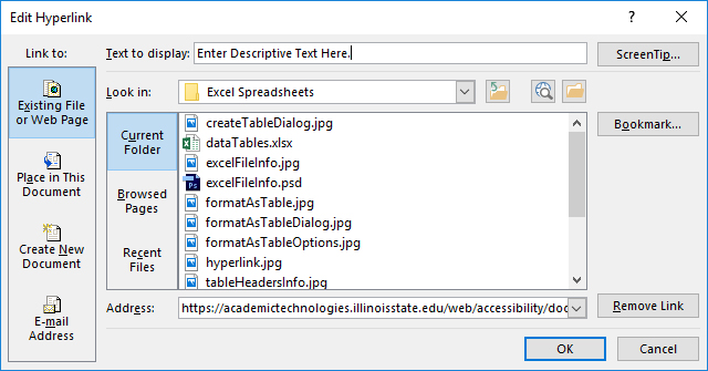
Step 1. Right click on Hyperlink
Rick click on URL hyperlink then select Edit Hyperlink from drop down.

Step 2. Enter descriptive Text.
Type Descriptive text (i.e. purpose or target of the link) into the Text to Display field.
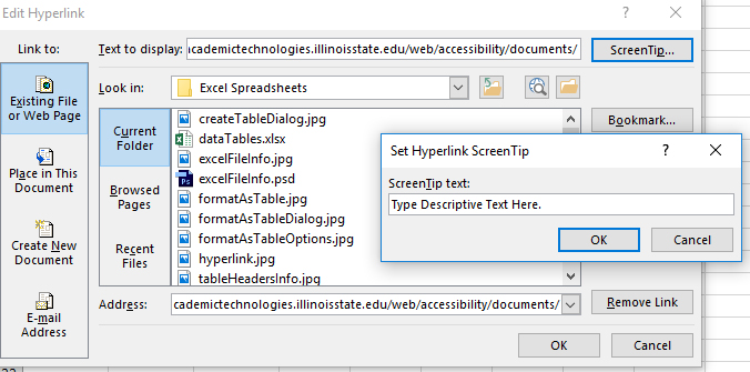
Note: If it is not possible to use descriptive link language in the Text to Display use the full URL, but add a ScreenTip. The Add a ScreenTip option is located to the right of the Text to Display field.
Set a Print Area
Hide all extra rows and columns outside the area being used to define the print area. This designates what cells to print when you don't want to print an entire worksheet. At the same time, setting the print area allows assistive technology users and keyboard-only users the ability to work only within the spreadsheet's data, and helps to keep them from getting lost in the unnecessary blank cells of the spreadsheet.
Step 1. Select First Empty Row or Column.
To hide rows and columns, select the first empty row or column closest to your data.

Step 2. Shift+End
Hold the Shift Key down and press and release the End Key on your keyboard. Don't let go of the Shift key.
Step 3. Right or Down Arrow
While still holding the Shift key press the Right Arrow to select all the blank columns to the end of the spreadsheet (use Down Arrow to select the blank rows). Keep holding down the Shift key.
Step 4. F10+H
Press and release the F10 key to open options drop down menu. Choose Hide (or press the H key) to hide all the blank cells. You can release the Shift key now.

Run the Accessibility Checker
Run the Microsoft Accessibility Checker.