Accessibility
Creating Accessible Data Tables in Microsoft Excel
Last modified 2/16/2022
When designing data tables it is important to remember that not everyone is able see the structure of the table and may need help the understand how the data is being presented. Oftentimes a data table may be used as an alternative text for complex images, graphs, or charts so it must to be accessible to assistive technologies. To ensure the the whole workbook is formatted, see Creating Accessible Excel Spreadsheets.
When possible, avoid:
- Merged cells
- Blank cells
Designing a New Table
Step 1. Select the cells.
Select the cells you want to include in your data table.
Step 2. Insert Table
From the Insert Tab, then select Tables group, and choose Table. In the Create Table Dialog box, check the checkbox to the left of My Table has Headers. Doing so will format the first row of the table as a header for each column. Choose OK.

Step 3. Enter Headers.
Excel creates a header row with the default names Column1, Column2, and so on. Replace the column header text in the first cell of each column with your descriptive header text. If your first column is also considered a header, check the checkbox to the left of First Column in the Table Tools Design Tab. Type new and descriptive names for each header cell.

Step 4. Add Your Data.
Type your data into your table.
Fixing Existing Simple Data Tables
If you are trying to improve the accessibility of an existing simple data table in Excel be sure the table has been formatted as a table.
Step 1. Format As Table
Select all the cells of your table then choose Format As Table from the Styles Ribbon on the Home Tab at the top of the page. A drop down of table style choices will appear. Remember to choose colors carefully when selecting your style.
Note: If you want to design a custom table style, choose the option for New Table Style. You can choose your own style and a custom option will be saved to the Format As Table Options.

Step 2. Check My Table has Headers
Once you choose a style the Format as Table dialog box will appear. Check the checkbox to the left of My Table has Headers. Doing so will format the first row of the table as a header. Choose OK.

Step 3. Specify Other Header Types
Place your cursor in the newly formatted table and a new Table Tools Tab should appear at the top of the screen. Select the Table Tools Tab and notice the checkbox to the left of Header Row is now checked. If your first column is also considered a header, check the checkbox to the left of First Column.

Step 4. Enter Table Name
In the Table Tools Design Tab, enter a Table name in the field provided. The table name should not have any spaces and should not be the same as any other table name in the workbook.

Coding Tables for Screen Readers
In order for screen readers to read the data tables in Excel, you need to add a piece of code to the Name Manager to tell it how the table is set up. To prepare this code, you need to answer some questions before entering the code.
Is this the first and only table on the worksheet?
If yes, write down the number 1. If no, write down the number of the table. Start counting your tables from the top of the spreadsheet.
What are the cell addresses for the top left and bottom right cells?
The cell address is made up of the column and row coordinates. Columns have letters associated to them and rows have numbers. To find the cell addresses for the table, locate the top left most corner of the table abd the bottom right cell including the table headers. Note which column letters and row numbers you are in.
For example, in the picture below the first cell in the table is located in the first column and the second row. The cell address is A2. The bottom right corner of the table is in cell C8. Once you select a cell, the cell address will also appear in a box in the top right corner of the spreadsheet.

What worksheet is the table located on ?
Note the number of the worksheet the table is on. Count left to right in the workbook.

Don't forget to give your worksheets descriptive names.
Does this table have a column header, a row header, or both?
Column Header
The top row has the header information. This type of header is referred to as a "ColumnTitleRegion" in Excel.

Row Header
The first column has the header information. This type of header is referred to as a "RowTitleRegion" in Excel.

Both Column and Row Headers
Both the first row and the first column have header information. This type of header is referred to as a "TitleRegion" in Excel.

Putting Together the Title Region Codes
The Title Region code is made up from the answers to the above Questions.
[Type of Header][Table Number].[Top Left Cell Address].[Bottom Right Cell Address].[Worksheet Number]
The code should not have any spaces between words, numbers or punctuation. Capitalize the first letters in the words Title, Region, Column and Row. This code is case sensitive.
Example Codes
- My table has only column headers
ColumnTitleRegion[table number].[top left cell address].[bottom right cell address].[worksheet number]
Example:

ColumnTitleRegion1.a16.e19.1
- My table has only row headers
RowTitleRegion[table number].[top left cell address].[bottom right cell address].[worksheet number]
Example:

RowTitleRegion1.a10.b14.1
- My table has both column and row headers
TitleRegion[table number].[top left cell address].[bottom right cell address].[worksheet number]
Example:
TitleRegion1.a16.e19.1
Add Title Region Code to Name Manager
Add Title Region Code to Name Manager
To add the Title Region code to the Name Manager. Select the top left cell in the table. Navigate to and select the Formulas tab in the Ribbon. In the Define Names group, choose the Name Manager option.

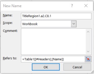
In the Name Manager dialog, choose the New button.

In New name dialog, type in the Title Region code in the Name edit box. Ignore other fields in the New name dialog. Choose OK button.